Dataset Drift Controls Using Raw Image Data and Differentiable ISPs
From Raw to Logit
Code  Data
Data ![]() Experiment server
Experiment server 
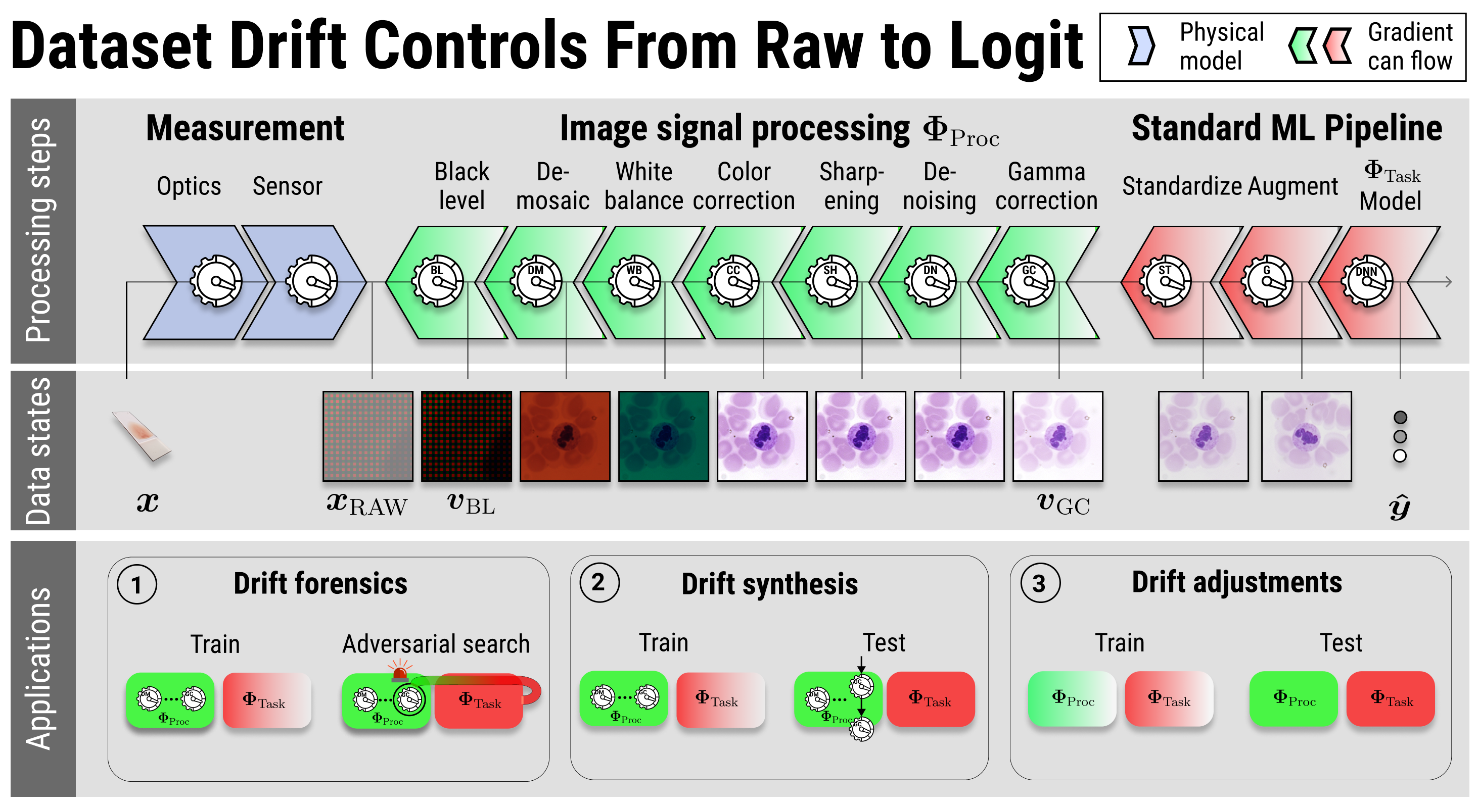
To create an image, raw sensor data traverses complex image signal processing pipelines. These pipelines are used by cameras and scientific instruments to produce the images fed into machine learning systems. The processing pipelines vary by device, influencing the resulting image statistics and ultimately contributing to what is known as hardware-drift. However, this processing is rarely considered in machine learning modelling, because available benchmark data sets are generally not in raw format. Here we show that pairing qualified raw sensor data with an explicit, differentiable model of the image processing pipeline allows to tackle camera hardware-drift. Specifically, we demonstrate (1) the controlled synthesis of hardware-drift test cases, (2) modular hardware-drift forensics, as well as (3) image processing customization. We make available two data sets. The first, Raw-Microscopy, contains 940 raw bright-field microscopy images of human blood smear slides for leukocyte classification alongside 5,640 variations measured at six different intensities and twelve additional sets totalling 11,280 images of the raw sensor data processed through different pipelines. The second, Raw-Drone, contains 548 raw drone camera images for car segmentation, alongside 3,288 variations measured at six different intensities and also twelve additional sets totalling 6,576 images of the raw sensor data processed through different pipelines.
In order to address camera hardware-drift we require two ingredients: raw sensor data and an image processing model. In the following we explain how the Raw-Microscopy and Raw-Drone datasets were collected for this study and how the processing model is built.
Raw data
Raw-Microscopy
Assessment of blood smears under a light microscope is a key diagnostic technique
Raw-Drone
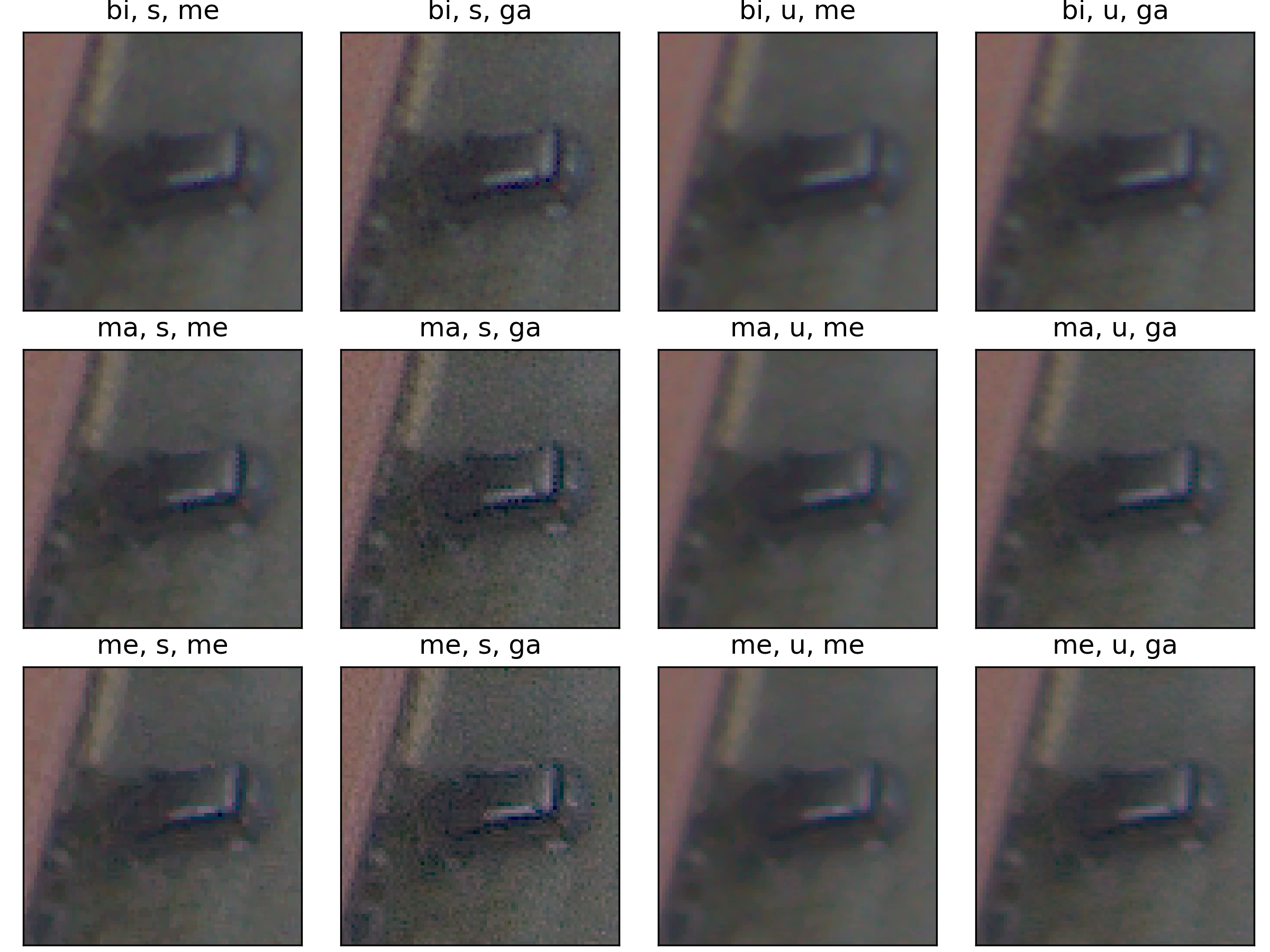
We used a DJI Mavic 2 Pro Drone, equipped with a Hasselblad L1D-20c camera (Sony IMX183 sensor) having 2.4 $\micro$m pixels in Bayer filter array. The objective has a focal length of 10.3 mm. We set the f-number \(N=8\), to emulate the PSF circle diameter relative to the pixel pitch and ground sampling distance (GSD) as would be found on images from high-resolution satellites. The point-spread function (PSF) was measured to have a circle diameter of 12.5$\micro$m. This corresponds to a diffraction-limited system, within the uncertainty dominated by the wavelength spread of the image. Images were taken at 200 ISO, a gain of 0.528 DN/$e^-$. The 12-bit pixel values are however left-justified to 16-bits, so that the gain on the 16-bit numbers is 8.448 DN/$e^-$. The images were taken at a height of 250 m, so that the GSD is 6 cm. All images were tiled in 256 \(\times\) 256 patches. Segmentation color masks were created to identify cars for each patch. From this mask, classification labels were generated to detect if there is a car in the image. The dataset is constituted by 548 images for the segmentation task, and 930 for classification. The dataset is augmented through JetRaw Data Suite, with 7 different intensity scales.
The second ingredient to our experiments is the image processing model which we describe next.
Lens2Logit - The image processing framework
Let $(X,Y):\Omega \to \mathbb{R}^{H,W}\times \mathcal{Y}$ be the raw sensor data generating random variable on some probability space $(\Omega, \mathcal{F},\mathbb{P})$, with $\mathcal{Y}={0,1}^{K}$ for classification and $\mathcal{Y}={0,1}^{H,W}$ for segmentation. Let $\Phi_{Task}:\mathbb{R}^{C,H,W}\to\mathcal{Y}$ be the task model determined during training. The inputs that are given to the task model $\state{\F}{Task}$ are the outputs of the image signal processing (ISP). We distinguish between the raw sensor image $\boldsymbol{x}$ and a view $\boldsymbol{v}=\state{\F}{Proc}(\boldsymbol{x})$ of this image, where $\state{\F}{Proc}\colon\R^{H,W}\to\R^{C,H,W}$ models the ISP. In contrast to the classical setting, this approach is more sensitive to the origin of distribution shifts, as outlined in our formal companion. We provide two explicit models for ISP: a static model $\Phi^{stat}_{Proc}$ and a parametrized model $\Phi^{\theta}_{Proc}$.
The static pipeline
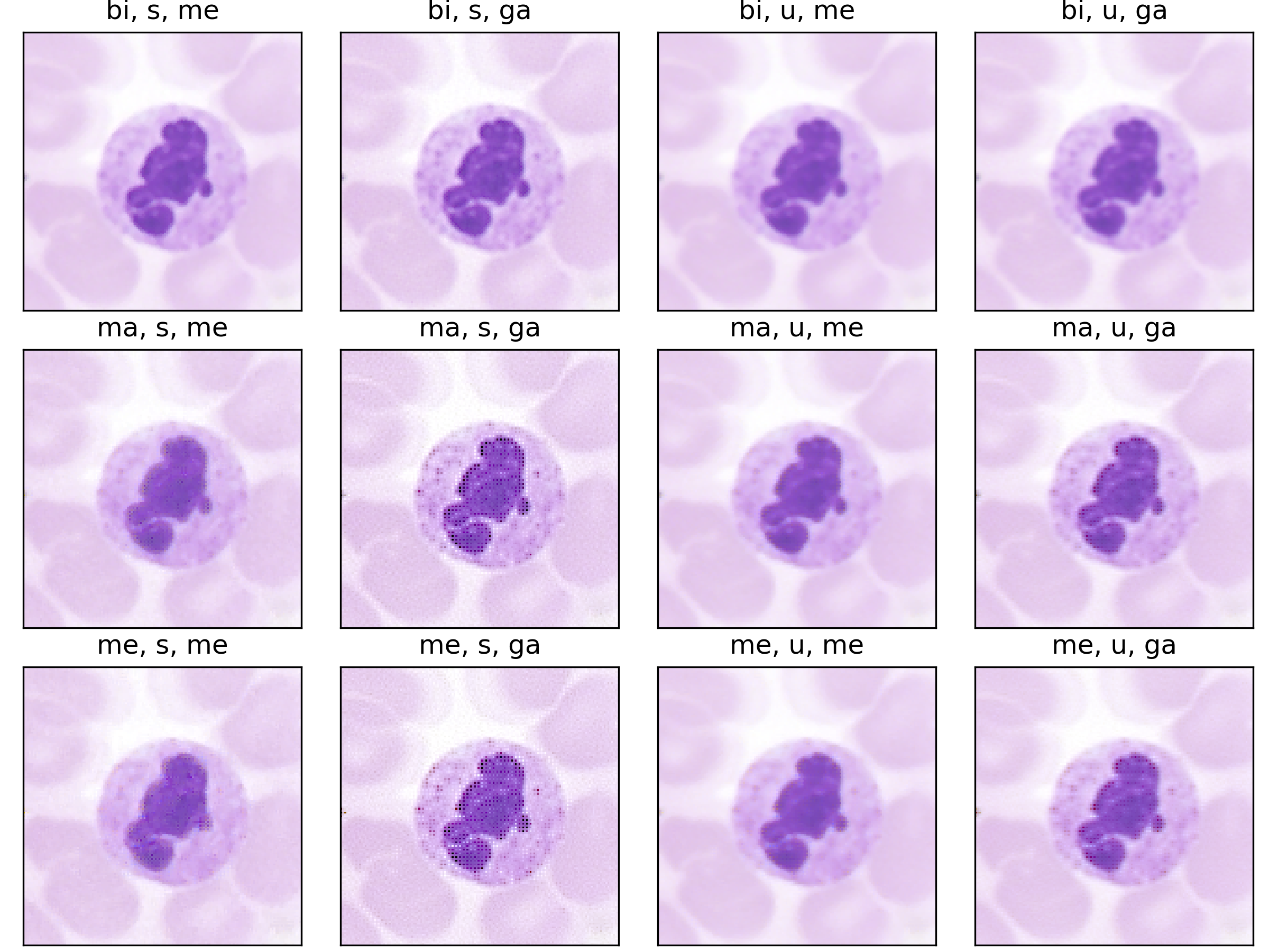
Following the most common steps in ISP, we define the static pipeline as the composition \(\begin{equation*} \Phi^{stat}_{Proc} := \Phi_{GC} \circ \Phi_{DN} \circ \Phi_{SH} \circ \Phi_{CC} \circ \Phi_{WB} \circ \Phi_{DM} \circ \Phi_{BL}, \end{equation*}\) mapping a raw sensor image to a RGB image. The static pipeline enables us to create (multiple) different views of the same raw sensor data by manually changing the configurations of the intermediate steps. Fixing the continuous features, but varying $\Phi_{DM}$, $\Phi_{SH}$ and $\Phi_{DN}$ results in the twelve different views visible further down in this post. For a detailed description of the static pipeline and its intermediate steps we refer to our formal companion.
The parametrized pipeline
For a fixed raw sensor image, the parametrized pipeline $\Phi^{\theta}_{Proc}$ maps from a parameter space $\Theta$ to a RGB image. The parametrized pipeline is differentiable wrt. the parameters in $\boldsymbol{\theta}$. This enables us to backpropagate the gradient from the output of the task model through the ISP back to the raw sensor image. You can find more details in our formal companion.
With raw data and and a controllable processing pipeline in our hands we are able to do interesting things. We can synthesize different realistic views from our raw sensor data (like the ones shown above), perform hardware-drift forensics on machine learning model as well as customued image processing.
Resources
Data
Access
If you use our code you can use the convenient cloud storage integration. Data will be loaded automatically. We also maintain a copy of the entire dataset with a persistent and permanent identifier at Zenodo which you can find under identifier 10.5281/zenodo.5235536.
License
The data is published under a Attribution 4.0 International (CC BY 4.0) which allows liberal copying, redistribution, remixing and transformation. The authors bear all responsibility for the published data.
Code
Access
All code is available at the raw2logit repository.
License
The code is published under MIT license which permits broad commercial use, distribution, modification and private use.
Virtual lab log
We maintain a collaborative virtual lab log at this address. There you can browse experiment runs, analyze results through SQL queries and download trained processing and task models.
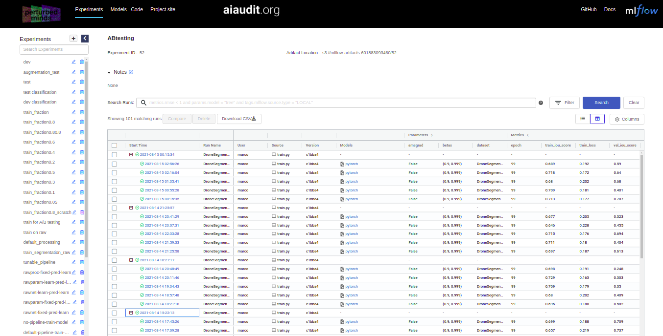
For better overview we include a map between the names of experiments in the paper and names of experiments in the virtual lab log:
| Name of experiment in paper | Name of experiment in virtual lab log |
|---|---|
| 5.1 Controlled synthesis of hardware-drift test cases | 1 Controlled synthesis of hardware-drift test cases (Train) , 1 Controlled synthesis of hardware-drift test cases (Test) |
| 5.2 Modular hardware-drift forensics | 2 Modular hardware-drift forensics |
| 5.3 Image processing customization | 3 Image processing customization (Microscopy), 3 Image processing customization (Drone) |
Note that the virtual lab log includes many additional experiments.